Previous Contents Next

3   Program normalization

The first step is always the construction of the DFG and transformation into a SARE. The reader is referred to [7] for a detailed account of this process.

3.1   Elimination of Variables Using Substitutions

As we have said, we want to keep the complexity of the pattern matching phase as low as possible. Our choice is to consider only one variable reductions. The price we pay for that is our inability to detect ``systems of reductions'', as Callahan does in the special case of linear recurrences. Now, computations often use temporary variables which lead to recurrences on several variables, therefore a system normalization must be provided to collapse multi-variables recurrences onto single-variable ones if possible. A similar situation occurs in the case of systems of first order differential equations:
x' = v,   v' = f(x) ,
which can be transformed into one second order differential equation x'' = f(x).

The recurrence defined by the system below is a two-variables one:
x[i] = case 
         i | i = 1  :       0 ;
         i | 2 <= i <= n  : y[i - 1] + a[i] ;
       esac ;
y[i] = case 
         i | i = 1  :       0 ;
         i | 2 <= i <= n  : x[i - 1] + b[i] ;
       esac ;

 
If our pattern matching is directly applied no scan can be detected since there is no self-referencing variable. Our solution is to eliminate either x or y from the system. For example if we replace the reference to y in x by its definition, the result is:
x[i] = case 
         i | i = 1  :       0 ;
         i | i = 2  :       0 ;
         i | 3 <= i <= n  : x[i - 2] + b[i - 1] + a[i] ;
       esac ;

 
The variable x is now self-referencing (with stride 2) and a mere pattern matching can point out that x is to be computed by summing the data b[i-1]+a[i]. Going from the first to the second system is not a simple textual substitution, We had to compute the expression y[i-1] from the definition of y in the initial system, then substitute it into the definition of x, then simplify the result by eliminating cases with empty domains. See [19] for details.
We also want our scan detector to handle scans on multi-dimensional arrays. In this context another problem arises: scans can be computed along very different paths in these arrays. The problem of detecting scans along arbitrary paths seems intractable, hence we deal only with rectilinear ones. An uni-directional scan gathers its data following one vector. An uni-directional scan associated with a multi-dimensional array represents in fact a set of scans:
The following program computes a set of scans along the diagonals of the array a:
DO i=1,n
 DO j=1,n
  a(i,j)=a(i-1,j-1)+a(i,j)
 END DO
END DO

 
The uni-directional scan underlying this code has direction (1 , 1) .
Several detection schemes can be used according to the required precision. The simplest algorithm consists in considering the system of equations as a whole and eliminating as many variables as possible. At this point most of the recurrences are defined by only one variable and a pattern matching can take place. The drawback of this method is that since, as we will see later, removing all circuits in a DFG is not always possible, unguided substitutions may lead into a blind alley, while a more sophisticated algorithm may have found a solution.

No scan can be extracted from the following system using this simple scheme:
x[i,j] = case
            i, j | i=1, j=1         :  0 ;
            i, j | 2<=i<=n, j=1     :  y[i-1,m] ;
            i, j | 1<=i<=n, 2<=j<=m :  x[i,j-1] + a[i,j] ;
          esac ;
y[i,j] = case
            i, j | 1<=i<=n, j=1     :  x[i,m] ;
            i, j | 1<=i<=n, 2<=j<=m :  y[i,j-1] + b[i,j] ;
          esac ;

 
But the third clause of x and the second of y compute sets of scans. In fact the elimination fails because the recurrences defined by this system are cross-referencing (cannot be computed in parallel).
A more complex detection scheme can be designed using multistage eliminations. The principle is to consider only some references (i.e. equations between our multi-dimensional variables). In a first stage only the references related to the innermost loops of the original program are taken into account. This is equivalent to considering the innermost loops as stand-alone programs in which the external loop counters are considered as fixed parameters. Pattern matching is then applied and closed forms are introduced for the detected scans. In the second stage we add to the graph the references relative to the loops just surrounding the innermost ones. A normalization and a pattern matching are performed again and so on. In this way the elimination is obviously more efficient and we can detect more complex scans (see section 4.1). Since closed forms appear during the detection process, pattern matching may be applied on variables already defined by a scan. In most cases this denote a scan whose path is piecewise rectilinear, a multi-directional scan.

Our previous example can be handled if the counter i relative to the outermost loop is considered as a parameter. In this context no elimination is to be performed since the only remaining references are the self-referencing ones in the last clauses of x and y. Let sum be the textual equivalent of the å operator, closed forms can be introduced for the scans:
x[i,j] = case
            i, j | i=1, j=1         :  0 ;
            i, j | 2<=i<=n, j=1     :  y[i-1,m] ;
            i, j | 1<=i<=n, 2<=j<=m :  x[i,1]+sum(j>=2,a(i,j)) ;
          esac ;
y[i,j] = case
            i, j | 1<=i<=n, j=1     :  x[i, m] ;
            i, j | 1<=i<=n, 2<=j<=m :  y[i,1]+sum(j>=2,b(i,j)) ;
          esac ;

 
It is very important to note that the closed forms are parametric with respect to i.
A technical issue for the multistage elimination scheme is the characterization of the references to be taken into account. At the SARE level, there is no longer information about the loop nests. We replace the missing information with the help of the concept of reference ``pseudo-depth''. Let the reference to a variable y in an equation for x be of the form:
" iÎ D, x(i)=...y(d(i))... .
where d is the dependence function. The pseudo-depth is the greatest integer p such that :
" iÎ D, d(i)[1..p]=i[1..p] .
Since dependence functions are supposed to be affine, the pseudo-depth can be obtained by formally computing the vector d(i) - i and counting its leading zero coordinates.

When normalizing loops strictly deeper than p, one has only to consider the references of pseudo-depth greater or equal than p.
Proof:
Only circuits of references can cause the elimination process to fail. The references of pseudo-depth greater or equal to p which are not references relative to the loops at a level strictly greater than p cannot be included in a circuit.
The following algorithm summarizes the steps of the multistage elimination method:
Algorithm 1  Scans Detection

3.2   Criterion for Total Elimination

The goal of our elimination phase is to collapse recurrences on several variables into recurrences on only one variable. The tool we use to perform the transformation is substitution. In this section we give a criterion for deciding if a SARE can be transformed into a single variable recurrence.

To introduce our proof let us consider a system of ordinary equations.

ì
ï
ï
ï
ï
ï
ï
ï
ï
ï
í
ï
ï
ï
ï
ï
ï
ï
ï
ï
î
x1=f1(x
 
k11
,...,x
 
k
1
 
m1
)
·
·
·
xi=fi(x
 
k1i
,...,x
 
k
i
 
mi
)
·
·
·
xn=fn(x
 
k1n
,...,x
 
k
n
 
mn
)
.
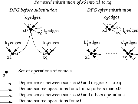
We do not make any assumption on the functions (fi)iÎN nor on the variables xi. In this context substitution is really the only operation we can use on the system. Such a system can be represented using a graph. The vertices are the n variables and there is an edge from xi to xj if xi appears in the definition of xj. Let us consider the effect of the substitution of x0 into x1, x2, ..., xq. The edges from x0 to the other vertices are removed and the k0 predecessors of x0 are added to the predecessors of the targets. Note that the new number of predecessors of, for instance, x1 is not exactly known. If we denote by k1 the initial number of predecessors of x1, it is only possible to say that the new number of predecessors k'1 is between max(k1,k0) and k1+k0: some of the predecessors of x0 may also be predecessors of x1, and are only counted once. Substitution for x0 eliminates it if the equation for x0 is not self recursive as shown on figure 2.


Figure 2: Effect of forward substitution on DFG


The substitution process terminates when no more variable can be eliminated. The process succeeds if, in the terminal system, all circuits are loops.

Theorem 2  [Sufficient Condition for a Total Elimination]   If the circuits of a strongly connected system 4 have a common vertex then the elimination process succeeds on the system.
Proof:
Without the edges going out of the common vertex the system graph is acyclic. Hence a topological sort can be performed on this sub-graph. The result of this sort is a partition of the vertices into sets S1,...,Sp. At this point one can substitute the definitions of the variables in S1 into the definitions of the variables in S2. These variables are now defined only in terms of the common vertex variable. Repeating the substitutions until Sp lead to a folding of all circuits into loops on the common vertex.
Theorem 3  [Necessary Condition for a Total Elimination]   The elimination process succeeds on a strongly connected system only if its circuits have a common vertex.
Proof:
The sketch of the proof is as follows. Let G be a strongly connected graph such that for each vertex v of G there is a circuit which does not include v. We show that a graph G' obtained from G by applying some substitutions include a strong component with the same properties as G. Moreover such a strong component has at least two vertices, hence it has a circuit of length greater or equal to 2.

Let us now detail the proof. The basic property of transformation by substitutions is that if v- is a predecessor of v in G, either v- or its predecessors in G are predecessor(s) of v in G'. This implies a conservation property on paths. More precisely if there is a path p in G, then there is a sub-path of p in G which starts with the first or the second vertex of p and stop at the last vertex of p. A special case arises when the path p is in fact a circuit. In this case there is at least one circuit in G' which includes only vertices from p. From the conservation property on paths and circuits, another conservation property can be deduced on inter-circuits paths. Let c1 and c2 be two circuits of G, for each circuit c'2 built from c2 in G', there is a path from a circuit built from c1 in G' to c'2.

Since each circuit of G' built from a circuit of G has as predecessor (via a path) at least one of the circuits of G' built from a given circuit of G (remember that G is strongly connected), there is in G' a strong component including at least one of the circuits of G' build from each circuit of G. For each vertex v of this strong component there exists a circuit of the component which does not include v. Indeed since v is not included in at least one circuit c of G, it is not included in the circuits of G' build from c (one of these is necessary in the strong component).
These results apply only to strongly connected systems but they can be adapted for other systems. It suffices to compute the strong components of the system and verify that each component fulfills the requirement. Our elimination criterion formalizes an intuitive thought: it is not always possible to solve a system of equations using only substitutions. The criterion is mostly interesting when nothing is known about the functions (fi)iÎN of the system (2). In other cases methods using more powerful operations than substitution are generally used to solve the system.
In the context of linear equations, systems such as (2) can always be solved. This is due to the fact that the Gaussian elimination algorithm use substitutions and also linear simplification. Linear simplification is a powerful tool since it can remove loops from the system graph. For example in the graph of the system below there is a loop on the vertex x1:
ì
í
î
x1=4.x1+x2
x2=2.x1
.
After simplification of the first equation (x1=-1/3x2) there is no longer a loop on x1.
The criterion is also valid for a SARE. Its graph is more complex since some edges are defined only in a sub-domain of the variable definition domain. This has an influence on the elimination process. After a substitution, new edges domains are computed by intersection of the old domains. If this intersection is void, the edge does not really exist. Hence the criterion is always sufficient but no longer necessary. One may also say that the criterion is sufficient and necessary if no simplification of the clause domains occurs.

3.3   Algorithms for Variables Elimination

All algorithms for variable elimination on strongly connected components have the same pattern: find the common vertex of the system graph circuits and use a topological sort to schedule the substitutions (as described in theorem (2)). Hence the difficult point is to find the common vertex.

There is a full range of algorithms to perform this operation. Let us begin with a heuristic method, which is not very efficient but very fast. We use the fact that a graph without cycles is also without circuits 5. Hence to find a vertex included in each circuit of a graph G, it suffices to consider each vertex v of G, to remove its outgoing edges and verify that the remaining graph Gv is acyclic. This verification can be done using the cyclomatic number 6 n(Gv)=m'-n'+p', with m' the number of edges of Gv, n' the number of vertices of Gv (the same as the number n of vertices of G) and p' its number of connected components (i.e. 1 since Gv is a connected graph). The number of edges m' of Gv is the number of edges m of G minus the number mv of v successors. Hence one has to check for each vertex v if the expression m-mv-n+1 is zero. The test complexity is about O(n) but it is only a heuristic since it does not discriminate between cycles and circuits.

This heuristic can be transformed into an exact method. It suffices to replace the computation of the cyclomatic number by a depth-first search to insure that there is no circuit in the graph. This method complexity is of the order of O(n.m).

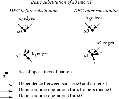
A more efficient way for elimination is to use basic substitutions. Basic substitutions are substitutions for variables which have only one successor. The effect of a basic substitution on the DFG of a system is depicted on figure 3.


Figure 3: Effect of basic forward substitution on DFG


If a basic substitution is applied to a strongly connected graph, there is no circuit including x0 and the resulting graph restricted to all vertices but x0 is also strongly connected.
Proof:
The vertex x0 has no longer successors, so no circuit can include this vertex. Moreover if a path exists between two vertices (different from x0) before the substitution, it also exists also after (even if the former includes x0, since it goes through x1 after the substitution).
When no basic substitution can be applied to a graph, either its strong component is reduced to a vertex and, in the initial graph, every circuit include this vertex, or the strong component includes several vertices and a total elimination cannot be performed on the initial graph.
Proof:
If the strong component is a single vertex, the elimination criterion implies that in the initial graph the circuits have a common vertex. Moreover the conservative property on circuits enforces that this vertex is the one in the strong component.

Let G' be a graph obtained from a strongly connected graph G using a basic substitution. Due to the properties of basic substitutions, if the strong component of G' is such that for each of its vertices v there exists a circuit not including v, then G has the same property. Now consider the final component including several vertices. No more basic substitution can be applied, hence each vertex has at least two successors. If a vertex v is removed, the others have still at least one successor, so there exists a circuit which does not include v.
This prove that the sequential application of basic substitutions is as powerful as the application of multiple substitutions in the context of our variable elimination process. An efficient algorithm can be extracted from the method provided that, for each vertex v, a sorted list of its predecessors pred(v) is available.
Algorithm 4  Finding a Common Vertex
  1. For each vertex v, compute its number of successors ns(v) and store one of these in succ(v).
  2. Initialize the stack s with the vertices having a unique successor.
  3. Stop if s is empty or if there is only one vertex in the component.
  4. Unstack v from s. Let v+ be the successor in succ(v).
  5. Perform a sorting merge on pred(v) and pred(v+), for each v- belonging to both lists subtract one to its number of successors ns(v-). When this number is equal to one stack v- on s.
  6. Store the result of the merging in pred(v+) and for each v- reset its peculiar successor succ(v-) to v+.
  7. Goto step 3.
The complexity of this algorithm is about O(n.d-) with n the number of vertices in the graph and d- the maximum size of the pred lists. So it may even be linear if, for instance, the graph is a mere circuit.

One may remark that finding the common vertex of the system graph circuits is the instance k = 1 of the problem of finding the minimum cutset of size less or equal to k. Hence any one of the algorithms for finding minimal cutsets which find every cutset of size 1 are suitable for variable elimination. That excludes algorithm D of Shamir, but the one described in [11] is perfect. In fact, it works for cutsets of size 1 and it finds minimal cutsets for a number of graph classes. This last property is important since even a partial elimination is useful: one obtains a system with less variables, which can be analyzed faster by the later phases of the automatic parallelization process (e.g. scheduling).

Note that a better variable elimination can be achieved using a more precise system graph: the clause graph (whose vertices are clauses and not variables).
The system associated to the program below
DO i=1,2*n
  a(i)=a(2*n-i+1)
END DO

 
is
x[i] = case 
         i | 1<=i<=n      : a[2*n-i+1] ;
         i | n+1<=i<=2*n  : x[2*n-i+1] ;
       esac ;
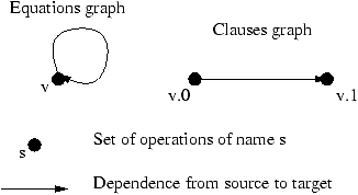
 
We name the clauses using the name of the variable and their rank in the variable definition. For instance the first clause of x is x.0. If x is included in a strong component, an elimination process may fail because of the loop in the variable graph. In contrast the clause graph does not have this loop, and so the elimination process may go further (see figure 4).


Figure 4: Example of difference between equation graph and clause graph


Previous Contents Next